

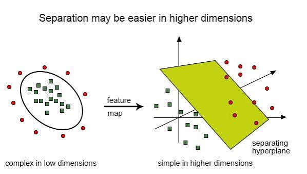
Some classification problems cannot be solved by drawing a straight line. When data points belonging to different classes are arranged in patterns that no linear boundary can separate — concentric circles, interlocking spirals, overlapping clusters — standard linear classifiers fail. Kernel methods are the mathematical framework developed to handle exactly this situation. Rather than abandoning linear classification altogether, kernel methods transform the data into a higher-dimensional space where a linear boundary does exist, then apply classification in that transformed space. The remarkable aspect is that this transformation happens implicitly — without ever computing the actual coordinates of the transformed points. For learners working through a data analytics course that covers supervised learning in depth, kernel methods represent one of the most mathematically elegant ideas in the field.
The Core Problem: When Linear Separation Is Impossible
A linear classifier — a Support Vector Machine (SVM) with a linear kernel, logistic regression, or a perceptron — finds a hyperplane that separates two classes in the original feature space. For two-dimensional data, this is simply a line. For three-dimensional data, it is a plane. The fundamental requirement is that the classes can be separated by such a flat boundary.
This requirement fails frequently in practice. Consider a dataset where class A occupies a central circular region and class B surrounds it. No straight line separates them. This configuration is called linearly inseparable, and it appears in domains ranging from image classification to genomics.
The conceptual resolution is straightforward: if the data cannot be separated in its current space, map it to a higher-dimensional space where it can. Adding a new feature — the squared distance from the origin, for example — can transform a circular boundary in two dimensions into a linear boundary in three. Once that boundary is found in the higher-dimensional space, it maps back to a curved boundary in the original space, correctly separating the classes.
The practical obstacle is computational. Explicitly computing new features for a high-dimensional transformation is expensive, and some transformations require infinite-dimensional spaces, making explicit computation impossible. Kernel methods resolve this through what is known as the kernel trick.
The Kernel Trick: Computing Without Transforming
The kernel trick is based on a specific observation: many learning algorithms — particularly SVMs — do not require the actual coordinates of data points in the transformed space. They only require the dot products between pairs of transformed points. A dot product measures the geometric similarity between two vectors.
A kernel function K(x, z) computes this dot product directly from the original feature values of two points x and z, without ever explicitly computing their transformed representations. This means the algorithm behaves as if it were operating in a high-dimensional feature space, while all computation remains in the original, lower-dimensional space.
The most widely used kernel functions are:
- Polynomial Kernel: K(x, z) = (xᵀz + c)^d — captures feature interactions up to degree d
- Radial Basis Function (RBF) / Gaussian Kernel: K(x, z) = exp(−γ‖x − z‖²) — implicitly maps to infinite-dimensional space; the most commonly used kernel in practice
- Sigmoid Kernel: Connects SVMs to neural network formulations
- Linear Kernel: No transformation; equivalent to standard linear classification
The RBF kernel is particularly notable. Its implicit feature space is infinite-dimensional, yet every computation involving it requires only the Euclidean distance between two points in the original space — a quantity that is cheap to compute regardless of how many features the data has.
Real-life use case: In bioinformatics, kernel SVMs have been applied to protein function prediction tasks where amino acid sequences must be classified by functional category. A 2004 study published in Bioinformatics demonstrated that string kernels — designed specifically for sequence data — outperformed standard feature-engineering approaches by classifying proteins with accuracy exceeding 90% on benchmark datasets. The kernel encoded biological similarity between sequences without requiring explicit feature extraction, a task that would have been computationally prohibitive otherwise.
This is precisely the kind of applied context that participants in a data analyst course in Vizag benefit from examining: the technique is not an abstraction — it is a deployed solution to a real computational constraint.
Kernel SVMs in Practice: Parameters, Trade-offs, and Applications
The most common application of kernel methods is the kernel Support Vector Machine. In addition to the choice of kernel, two parameters govern its behaviour:
- C (regularisation parameter): Controls the trade-off between maximising the margin — the gap between the decision boundary and the nearest data points — and minimising misclassification on the training set. A low C allows more misclassifications in exchange for a wider, more generalisable margin. A high C fits the training data more tightly but risks overfitting.
- γ (gamma, for RBF kernel): Controls the reach of individual training points. A high gamma means each point influences only its immediate neighbourhood, producing a tighter, more complex boundary. A low gamma produces smoother boundaries with broader influence.
These parameters are typically selected through cross-validated grid search — a standard practice covered in any comprehensive data analytics course that addresses model selection.
Real-life use case: Handwritten digit recognition was one of the early benchmark tasks where kernel SVMs demonstrated state-of-the-art performance. Applied to the MNIST dataset — 60,000 labeled handwritten digits — RBF kernel SVMs achieved error rates below 1.4% before deep learning methods superseded them. Their performance on this task validated the practical value of implicit high-dimensional feature mapping for image classification.
Real-life use case: In financial fraud detection, kernel SVMs have been used to classify transaction patterns where fraudulent and legitimate transactions overlap in ways that linear models cannot resolve. A 2018 study on credit card fraud detection found that RBF kernel SVMs achieved an area under the ROC curve (AUC) of 0.97 on a dataset of 284,807 transactions — outperforming logistic regression by a margin of approximately 4% on the same data, attributable specifically to the non-linear decision boundary the kernel enabled.
Limitations and When Kernel Methods Are Appropriate
Kernel methods carry specific computational and practical limitations that determine when they are suitable.
Scalability: The kernel matrix — which stores dot products between every pair of training points — grows quadratically with dataset size. For a dataset of 100,000 points, this matrix has 10 billion entries. Standard kernel SVMs are generally considered practical for datasets up to approximately 100,000 samples; beyond that, approximation methods such as the Nyström approximation or Random Fourier Features are required.
Kernel selection: No universal rule determines which kernel to use for a given problem. RBF is a robust default, but domain structure — sequences, graphs, images — may benefit from purpose-built kernels. This is an active research area, with custom kernels designed for text, biological sequences, and graph-structured data all demonstrating measurable performance gains over generic alternatives.
Interpretability: Unlike decision trees or logistic regression, kernel SVMs do not produce easily interpretable decision rules. The classification of any point depends on its kernel similarity to a set of support vectors — the training points closest to the decision boundary — which are meaningful to specialists but opaque in general business contexts.
Kernel methods are best suited for small to medium-sized datasets with complex, non-linear class boundaries, where accuracy is prioritised over interpretability and computational efficiency. For learners in a data analyst course in Vizag building a complete picture of classification methods, kernel SVMs occupy a specific and well-defined position: they are the principled solution to non-linearity that requires neither the depth of neural networks nor the simplicity of decision trees.
Concluding Note
Kernel methods address one of the most fundamental constraints in machine learning — the inability of linear classifiers to handle non-linearly separable data — through a mathematically efficient solution: computing similarity in a high-dimensional feature space without ever explicitly constructing it. The kernel trick makes this computationally feasible, and the RBF kernel in particular has proven robust across domains from image recognition to genomics to financial fraud detection.
Understanding kernel methods requires engaging with concepts that connect linear algebra, geometry, and statistical learning — which is precisely what makes them a valuable area of study. For anyone progressing through a data analytics course that covers classification in depth, kernel methods mark the boundary between foundational and advanced machine learning. They reward careful study with a framework that clarifies why neural networks work, how similarity-based learning scales, and what it means for a learning algorithm to be both powerful and principled.
